![]()
The goal of BiostatsUHNplus is to house publicly available code functions and snippets (some with multiple package dependencies) used by Biostatistics@UHN in Toronto, Canada.
Many of these functions build upon the features of reportRmd.
First, install the latest version of reportRmd from CRAN with:
Then install the latest version of BiostatsUHNplus from CRAN with:
If version 0.1.0 or higher of reportRmd is installed, the development version of BiostatsUHNplus can be installed from GitHub with:
# install.packages("devtools")
devtools::install_github("biostatsPMH/BiostatsUHNplus", ref="development")library(BiostatsUHNplus);
z <- as_numeric_parse(c(1:5, "String1",6:10,"String2"))
#> The following entries were converted to NA values:
#> Entry 6, 'String1'
#> Entry 12, 'String2'
z
#> [1] 1 2 3 4 5 NA 6 7 8 9 10 NAUses addendum simulated study data and applies variable labels. Interpret summary output and unnested or nested p-value with caution!
Note that if participants were enrolled in more than one cohort (crossover), or if repeat AEs in participant had different attribution, the total N for Full Sample will be less than that of the total N of attribution for first study drug. Since total N for Full Sample (234) is less than total N of the first study drug attribution categories (49 + 198), this suggests that there was instances of repeat AEs in participants having different attribution to first study drug.
library(plyr);
library(BiostatsUHNplus);

data("enrollment", "demography", "ineligibility", "ae");
clinT <- plyr::join_all(list(enrollment, demography, ineligibility, ae),
  by = "Subject", type = "full");
clinT$AE_SEV_GD <- as.numeric(clinT$AE_SEV_GD);
clinT$Drug_1_Attribution <- "Unrelated";
clinT$Drug_1_Attribution[clinT$CTC_AE_ATTR_SCALE %in%
                           c("Definite", "Probable", "Possible")] <- "Related";
clinT$Drug_2_Attribution <- "Unrelated";
clinT$Drug_2_Attribution[clinT$CTC_AE_ATTR_SCALE_1 %in%
                           c("Definite", "Probable", "Possible")] <- "Related";
lbls <- data.frame(c1=c("AE_SEV_GD", "ENROL_DATE_INT", "COHORT", "GENDER_CODE",
  "INELIGIBILITY_STATUS", "AE_ONSET_DT_INT", "Drug_2_Attribution", "ae_category"),
  c2=c("Adverse event severity grade", "Enrollment date", "Cohort", "Gender",
       "Ineligibility", "Adverse event onset date", "Attribution to second study drug",
       "Adverse event system organ class"));
clinT <- reportRmd::set_labels(clinT, lbls);

rm_covsum_nested(data = clinT, id = c("ae_detail", "Subject", "COHORT"),
  covs = c("COHORT", "GENDER_CODE", "INELIGIBILITY_STATUS", "ENROL_DATE_INT",
           "AE_SEV_GD", "Drug_2_Attribution", "AE_ONSET_DT_INT", "ae_category"),
maincov = "Drug_1_Attribution");| Full Sample (n=234) | Related (n=49) | Unrelated (n=198) | Unnested p-value | Unnested Effect Size | Unnested StatTest | Nested p-value | |
|---|---|---|---|---|---|---|---|
| Cohort | 0.65 | 0.081 | Chi Sq, Cramer’s V | 0.95 | |||
| Cohort A | 59 (25) | 13 (27) | 49 (25) | ||||
| Cohort B | 83 (35) | 14 (29) | 74 (37) | ||||
| Cohort C | 37 (16) | 10 (20) | 30 (15) | ||||
| Cohort D | 55 (24) | 12 (24) | 45 (23) | ||||
| Gender | 0.14 | 0.093 | Chi Sq, Cramer’s V | 0.63 | |||
| Female | 51 (22) | 15 (31) | 39 (20) | ||||
| Male | 183 (78) | 34 (69) | 159 (80) | ||||
| Ineligibility | Chi Sq, Cramer’s V | ||||||
| No | 215 (100) | 46 (100) | 181 (100) | ||||
| Missing | 19 | 3 | 17 | ||||
| Enrollment date | Wilcoxon Rank Sum, Wilcoxon r | ||||||
| Mean (sd) | 2017-01-07 (301.8 days) | 2017-01-31 (322.7 days) | 2016-12-28 (294.3 days) | ||||
| Median (Min,Max) | 2016-09-14 (2016-01-18, 2018-05-16) | 2017-02-07 (2016-01-18, 2018-05-16) | 2016-09-14 (2016-01-18, 2018-05-16) | ||||
| Adverse event severity grade | 0.12 | 0.098 | Wilcoxon Rank Sum, Wilcoxon r | 0.97 | |||
| Mean (sd) | 1.8 (0.8) | 2.0 (0.9) | 1.7 (0.8) | ||||
| Median (Min,Max) | 1.5 (1.0, 5.0) | 2 (1, 4) | 1.5 (1.0, 5.0) | ||||
| Attribution to second study drug | <0.001 | 0.55 | Chi Sq, Cramer’s V | <0.001 | |||
| Related | 37 (16) | 28 (57) | 11 (6) | ||||
| Unrelated | 197 (84) | 21 (43) | 187 (94) | ||||
| Adverse event onset date | Wilcoxon Rank Sum, Wilcoxon r | ||||||
| Mean (sd) | 2017-11-03 (161.1 days) | 2017-10-01 (146.6 days) | 2017-11-10 (161.2 days) | ||||
| Median (Min,Max) | 2017-10-05 (2016-05-02, 2019-01-13) | 2017-09-07 (2017-03-18, 2018-11-24) | 2017-10-15 (2016-05-02, 2019-01-13) | ||||
| Adverse event system organ class | 0.003 | 0.42 | Chi Sq, Cramer’s V |
Did not converge; quasi or complete category separation |
|||
| Blood and lymphatic system disorders | 15 (6) | 6 (12) | 10 (5) | ||||
| Cardiac disorders | 6 (3) | 0 (0) | 6 (3) | ||||
| Ear and labyrinth disorders | 1 (0) | 0 (0) | 1 (1) | ||||
| Endocrine disorders | 1 (0) | 1 (2) | 0 (0) | ||||
| Eye disorders | 4 (2) | 0 (0) | 4 (2) | ||||
| Gastrointestinal disorders | 32 (14) | 16 (33) | 22 (11) | ||||
| General disorders and administration site conditions | 19 (8) | 1 (2) | 18 (9) | ||||
| Hepatobiliary disorders | 2 (1) | 0 (0) | 2 (1) | ||||
| Immune system disorders | 1 (0) | 0 (0) | 1 (1) | ||||
| Infections and infestations | 15 (6) | 5 (10) | 13 (7) | ||||
| Injury, poisoning and procedural complications | 4 (2) | 1 (2) | 4 (2) | ||||
| Investigations | 34 (15) | 12 (24) | 23 (12) | ||||
| Metabolism and nutrition disorders | 25 (11) | 3 (6) | 22 (11) | ||||
| Musculoskeletal and connective tissue disorders | 7 (3) | 0 (0) | 7 (4) | ||||
| Neoplasms benign, malignant and unspecified (incl cysts and polyps) | 1 (0) | 0 (0) | 1 (1) | ||||
| Nervous system disorders | 20 (9) | 3 (6) | 18 (9) | ||||
| Psychiatric disorders | 4 (2) | 0 (0) | 4 (2) | ||||
| Renal and urinary disorders | 5 (2) | 0 (0) | 5 (3) | ||||
| Reproductive system and breast disorders | 1 (0) | 0 (0) | 1 (1) | ||||
| Respiratory, thoracic and mediastinal disorders | 19 (8) | 1 (2) | 18 (9) | ||||
| Skin and subcutaneous tissue disorders | 13 (6) | 0 (0) | 13 (7) | ||||
| Vascular disorders | 5 (2) | 0 (0) | 5 (3) |
Uses addendum simulated study data. DSMB-CCRU AE summary tables in below code example can be found in the man/tables folder of BiostatsUHNplus package.
library(BiostatsUHNplus);
data("enrollment", "demography", "ineligibility", "ae");

## This does summary for all participants;
dsmb_ccru(protocol="EXAMPLE_STUDY",setwd="./man/tables/",
          title="Phase X Study to Evaluate Treatments A-D",
          comp=NULL,pi="Dr. Principal Investigator",
          presDate="30OCT2020",cutDate="31AUG2020",
          boundDate=NULL,subjID="Subject",subjID_ineligText=c("New Subject","Test"),
          baseline_datasets=list(enrollment,demography,ineligibility),
          ae_dataset=ae,ineligVar="INELIGIBILITY_STATUS",ineligVarText=c("Yes","Y"),
          genderVar="GENDER_CODE",enrolDtVar="ENROL_DATE_INT",ae_detailVar="ae_detail",
          ae_categoryVar="ae_category",ae_severityVar="AE_SEV_GD",
          ae_onsetDtVar="AE_ONSET_DT_INT",ae_detailOtherText="Other, specify",
          ae_detailOtherVar="CTCAE5_LLT_NM",ae_verbatimVar="AE_VERBATIM_TRM_TXT",
          numSubj=NULL)

## This does summary for each cohort;
dsmb_ccru(protocol="EXAMPLE_STUDY",setwd="./man/tables/",
          title="Phase X Study to Evaluate Treatments A-D",
          comp="COHORT",pi="Dr. Principal Investigator",
          presDate="30OCT2020",cutDate="31AUG2020",
          boundDate=NULL,subjID="Subject",subjID_ineligText=c("New Subject","Test"),
          baseline_datasets=list(enrollment,demography,ineligibility),
          ae_dataset=ae,ineligVar="INELIGIBILITY_STATUS",ineligVarText=c("Yes","Y"),
          genderVar="GENDER_CODE",enrolDtVar="ENROL_DATE_INT",ae_detailVar="ae_detail",
          ae_categoryVar="ae_category",ae_severityVar="AE_SEV_GD",
          ae_onsetDtVar="AE_ONSET_DT_INT",ae_detailOtherText="Other, specify",
          ae_detailOtherVar="CTCAE5_LLT_NM",ae_verbatimVar="AE_VERBATIM_TRM_TXT",
          numSubj=NULL)

## Does same as above, but overrides number of subjects in cohorts;
dsmb_ccru(protocol="EXAMPLE_STUDY",setwd="./man/tables/",
          title="Phase X Study to Evaluate Treatments A-D",
          comp="COHORT",pi="Dr. Principal Investigator",
          presDate="30OCT2020",cutDate="31AUG2020",
          boundDate=NULL,subjID="Subject",subjID_ineligText=c("New Subject","Test"),
          baseline_datasets=list(enrollment,demography,ineligibility),
          ae_dataset=ae,ineligVar="INELIGIBILITY_STATUS",ineligVarText=c("Yes","Y"),
          genderVar="GENDER_CODE",enrolDtVar="ENROL_DATE_INT",ae_detailVar="ae_detail",
          ae_categoryVar="ae_category",ae_severityVar="AE_SEV_GD",
          ae_onsetDtVar="AE_ONSET_DT_INT",ae_detailOtherText="Other, specify",
          ae_detailOtherVar="CTCAE5_LLT_NM",ae_verbatimVar="AE_VERBATIM_TRM_TXT",
numSubj=c(3,4,3,3))Uses addendum simulated study data. Shows timeline for onset of related AE after study enrollment. Can display up to 5 attributions. Time unit may be one of day, week, month or year.
Note that if more than one field is given for startDtVars (unique names required), each field is assumed to be specific start date for attribution in corresponding field order.
The below plot includes both AE category and AE detail in default colour and font scheme.
library(ggplot2);
library(BiostatsUHNplus);
data("enrollment", "ae");

p <- ae_timeline_plot(subjID="Subject",subjID_ineligText=c("New Subject","Test"),
                 baseline_datasets=list(enrollment),
                 ae_dataset=ae,
                 ae_attribVars=c("CTC_AE_ATTR_SCALE","CTC_AE_ATTR_SCALE_1"),
                 ae_attribVarsName=c("Drug 1","Drug 2"),
                 ae_attribVarText=c("Definite", "Probable", "Possible"),
                 startDtVars=c("ENROL_DATE_INT"),ae_detailVar="ae_detail",
                 ae_categoryVar="ae_category",ae_severityVar="AE_SEV_GD",
                 ae_onsetDtVar="AE_ONSET_DT_INT",time_unit="week")
ggplot2::ggsave(paste("man/figures/ae_detail_timeline_plot", ".png", sep=""), p,
                width=6.4, height=10, device="png", scale = 1.15);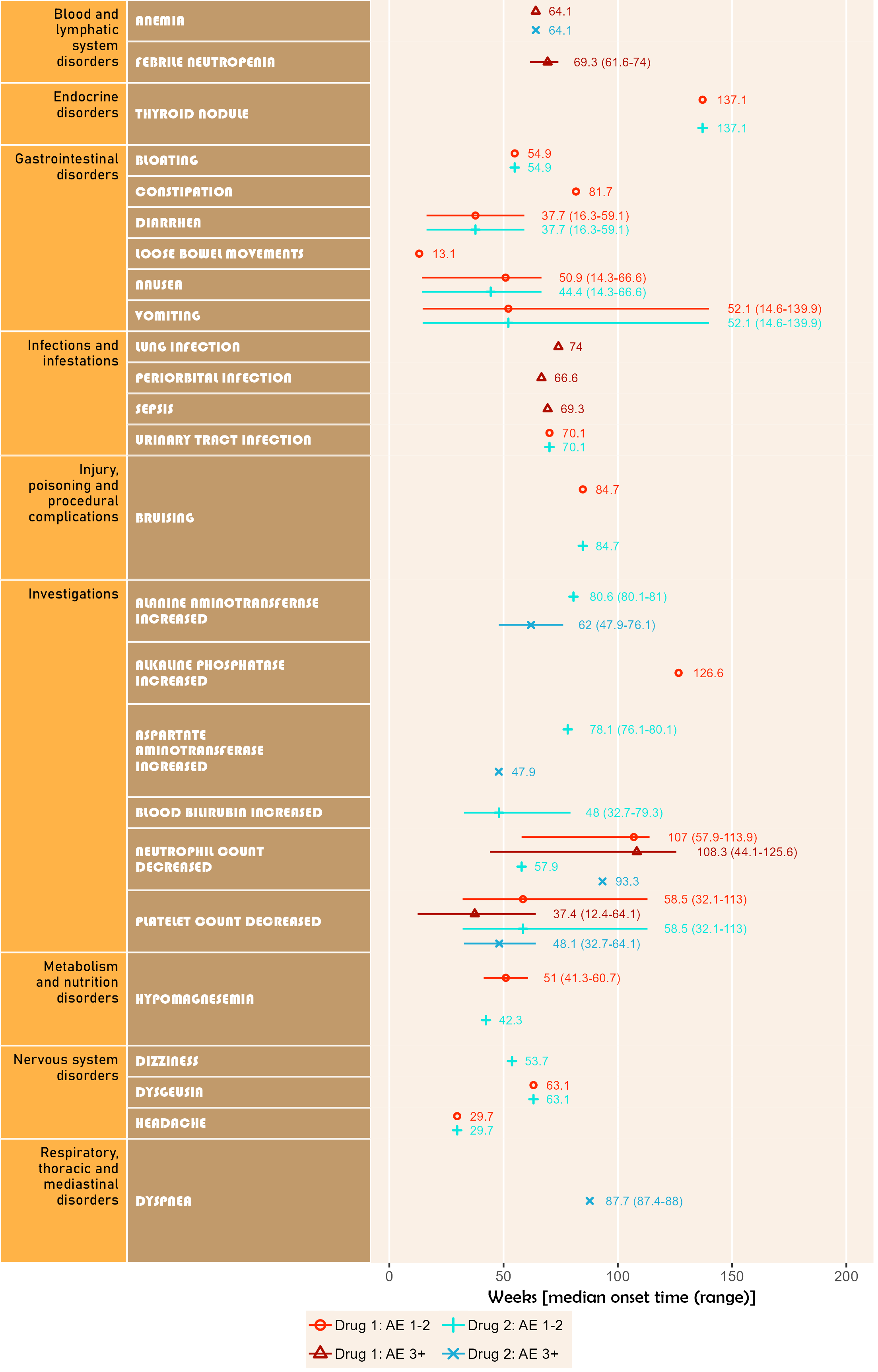
The next plot summarizes timeline by AE category. Fonts, colours, symbols, column widths (character length) and time unit are customized.
The width, height and scale parameters in ggsave() can also be modified to fit a large plot.
library(ggplot2);
library(BiostatsUHNplus);
data("enrollment", "ae");

p <- ae_timeline_plot(subjID="Subject",subjID_ineligText=c("New Subject","Test"),
                 baseline_datasets=list(enrollment),
                 ae_dataset=ae,
                 ae_attribVars=c("CTC_AE_ATTR_SCALE","CTC_AE_ATTR_SCALE_1"),
                 ae_attribVarsName=c("Drug 1","Drug 2"),
                 ae_attribVarText=c("Definite", "Probable", "Possible"),
                 startDtVars=c("ENROL_DATE_INT"),ae_detailVar="ae_detail",
                 ae_categoryVar="ae_category",ae_severityVar="AE_SEV_GD",
                 ae_onsetDtVar="AE_ONSET_DT_INT",time_unit="month",
                 include_ae_detail=FALSE,
                 fonts=c("Forte","Gadugi","French Script MT","Albany AMT","Calibri"),
                 fontColours=c("#FF4F00","#FFDB58"),
                 panelColours=c("#AAF0D1",NA,"white"),
                 attribColours=c("#F6ADC6","#C54B8C","#A4DDED","#0077BE","#9AB973",
                                 "#01796F","#FFA343","#CC7722","#E0B0FF","#5A4FCF"),
                 attribSymbols=c(5,6,7,8,15,16,17,18,19,20),
                 columnWidths=c(23,15))
ggplot2::ggsave(paste("man/figures/ae_category_timeline_plot", ".png", sep=""), p,
                width=3.6, height=5.4, device="png", scale = 1);
If available, specific start date for attribution in corresponding field order (unique field name required) can be used. Drug start date is closer to AE onset than enrollment date.
Below, subjects 01 and 11 are excluded.
library(ggplot2);
library(BiostatsUHNplus);
data("drug1_admin", "drug2_admin", "ae");

p <- ae_timeline_plot(subjID="Subject",subjID_ineligText=c("01","11"),
                 baseline_datasets=list(drug1_admin, drug2_admin),
                 ae_dataset=ae,
                 ae_attribVars=c("CTC_AE_ATTR_SCALE","CTC_AE_ATTR_SCALE_1"),
                 ae_attribVarsName=c("Drug 1","Drug 2"),
                 ae_attribVarText=c("Definite", "Probable", "Possible"),
                 startDtVars=c("TX1_DATE_INT","TX2_DATE_INT"),
                 ae_detailVar="ae_detail",
                 ae_categoryVar="ae_category",ae_severityVar="AE_SEV_GD",
                 ae_onsetDtVar="AE_ONSET_DT_INT",time_unit="month",
                 include_ae_detail=FALSE,
                 fonts=c("Calibri","Albany AMT","Gadugi","French Script MT","Forte"),
                 fontColours=c("#FFE135"),
                 panelColours=c("#E52B50",NA,"#FFF5EE"),
                 attribColours=c("#9AB973","#01796F","#FFA343","#CC7722"),
                 attribSymbols=c(7,8,5,6),
                 columnWidths=c(23))
ggplot2::ggsave(paste("man/figures/ae_category_attribStart_timeline_plot", ".png", sep=""),
                p, width=4.2, height=5.4, device="png", scale = 1);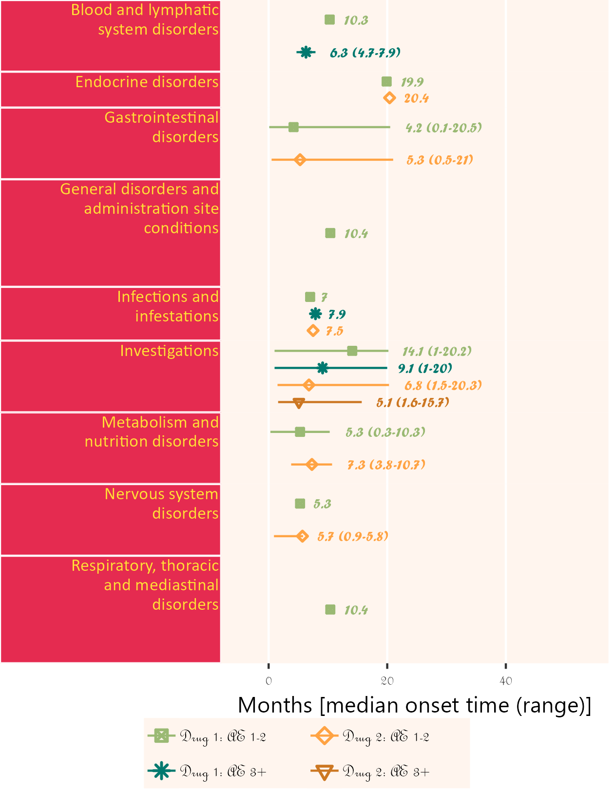
Below runs a logistic MCMCglmm model on the odds of grade 3 or higher adverse event, controlling for attribution of first and second intervention drugs. Subject and system organ class are treated as random effects. Model has 800 posterior samples. Should specify burnin=125000, nitt=625000 and thin=100 for 5000 posterior samples with lower autocorrelation. Aim for effective sample sizes of at least 2000.
data("ae");

ae$G3Plus <- 0;
ae$G3Plus[ae$AE_SEV_GD %in% c("3", "4", "5")] <- 1;
ae$Drug_1_Attribution <- "No";
ae$Drug_1_Attribution[ae$CTC_AE_ATTR_SCALE %in% c("Definite", "Probable", "Possible")] <- "Yes";
ae$Drug_2_Attribution <- "No";
ae$Drug_2_Attribution[ae$CTC_AE_ATTR_SCALE_1 %in% c("Definite", "Probable", "Possible")] <- "Yes";

prior2RE <- list(R = list(V = diag(1), fix = 1),
  G=list(G1=list(V=1, nu=0.02), G2=list(V=1, nu=0.02)));

model1 <- MCMCglmm::MCMCglmm(G3Plus ~ Drug_1_Attribution + Drug_2_Attribution,
  random=~Subject + ae_category, family="categorical", data=ae, saveX=TRUE,
  verbose=F, burnin=2000, nitt=10000, thin=10, pr=TRUE, prior=prior2RE);

mcmcglmm_mva <- nice_mcmcglmm(model1, ae);
options(knitr.kable.NA = '');
knitr::kable(mcmcglmm_mva);| Variable | Levels | OR (95% HPDI) | MCMCp | eff.samp |
|---|---|---|---|---|
| Drug 1 Attribution | No | reference | ||
| Yes | 2.77 (1.22, 6.93) | 0.022 | 193.23 | |
| Drug 2 Attribution | No | reference | ||
| Yes | 0.45 (0.16, 1.35) | 0.145 | 156.40 |
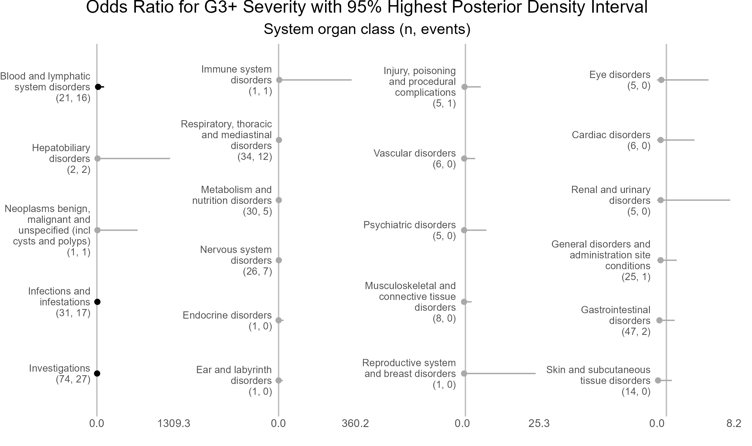
Most of the observed variation in grade 3 or higher adverse event status is attributable to adverse event category, also known as system organ class.
mcmcglmm_icc <- nice_mcmcglmm_icc(model1, prob=0.95, decimals=4);
options(knitr.kable.NA = '');
knitr::kable(mcmcglmm_icc);| ICC | lower | upper | |
|---|---|---|---|
| Subject | 0.0583 | 0.0068 | 0.3010 |
| ae_category | 0.8144 | 0.5145 | 0.9572 |
| units | 0.0725 | 0.0272 | 0.2458 |
After controlling for first and second drug attributions, subject 01 has a higher odds for grade 3 or higher adverse event than the average of study participants.
p <- caterpillar_plot(subjID = "Subject",
  mcmcglmm_object = model1,
  prob = 0.95,
  orig_dataset = ae,
  ncol = 2,
  binaryOutcomeVar = "G3Plus")
ggplot2::ggsave(paste("man/figures/caterpillar_plot_subject", ".png", sep=""),
       p, scale = 1.0, width=6.4, height=3.4, device="png");
Highest posterior density intervals, also known as credible intervals, are not symmetric. Need to run model for more iterations with higher burnin.
p <- caterpillar_plot(subjID = "ae_category",
  mcmcglmm_object = model1,
  prob = 0.95,
  orig_dataset = ae,
  ncol = 4,
  binaryOutcomeVar = "G3Plus",
  subtitle = "System organ class (n, events)",
  title = "Odds Ratio for G3+ Severity with 95% Highest Posterior Density Interval",
  fonts = c("Arial", "Arial", "Arial", "Arial"),
  break.label.summary = TRUE)
ggplot2::ggsave(paste("man/figures/caterpillar_plot_ae_category", ".png", sep=""),
       p, scale = 1.0, width=6.4, height=4.0, device="png");