![]()
mixvlmc implements variable length Markov chains (VLMC)
and variable length Markov chains with covariates (COVLMC), as described
in:
mixvlmc includes functionalities similar to the ones
available in VLMC
and PST. The main
advantages of mixvlmc are the support of time varying
covariates with COVLMC and the introduction of post-pruning of the
models that enables fast model selection via information criteria.
The package can be installed from CRAN with:
install.packages("mixvlmc")The development version is available from GitHub:
# install.packages("devtools")
devtools::install_github("fabrice-rossi/mixvlmc")Variable length Markov chains (VLMC) are sparse high order Markov
chains. They can be used to model time series (sequences) with discrete
values (states) with a mix of small order dependencies for certain
states and higher order dependencies for other states. For instance,
with a binary time series, the probability of observing 1 at time \(t\) could be constant whatever the older
past states if the last one (at time \(t-1\)) was 1, but could depend on states at
time \(t-3\) and \(t-2\) if the state was 0 at time \(t-1\). A collection of past states that
determines completely the transition probabilities is a context
of the VLMC. Read vignette("context-trees") for details
about contexts and context tree, and see
vignette("variable-length-markov-chains") for a more
detailed introduction to VLMC.
VLMC with covariates (COVLMC) are extension of VLMC in which transition probabilities (probabilities of the next state given the past) can be influenced by the past values of some covariates (in addition to the past values of the time series itself). Each context is associated to a logistic model that maps the (past values of the) covariates to transition probabilities.
The package is loaded in a standard way.
library(mixvlmc)
library(ggplot2)
The main function of VLMC is vlmc() which can be called
on a time series represented by a numerical vector or a factor, for
instance.
set.seed(0)
x <- sample(c(0L, 1L), 200, replace = TRUE)
model <- vlmc(x)
model
#> VLMC context tree on 0, 1
#>  cutoff: 1.921 (quantile: 0.05)
#>  Number of contexts: 11
#>  Maximum context length: 6
The default parameters of vlmc() will tend to produce
overly complex VLMC in order to avoid missing potential structure in the
time series. In the example above, we expect the optimal VLMC to be a
constant distribution as the sample is independent and uniformly
distributed (it has no temporal structure). The default parameters give
here an overly complex model, as illustrated by its text based
representation
draw(model)
#> * (0.505, 0.495)
#> '-- 1 (0.4848, 0.5152)
#>     +-- 0 (0.5319, 0.4681)
#>     |   '-- 1 (0.5, 0.5)
#>     |       '-- 0 (0.4444, 0.5556)
#>     |           '-- 0 (0.4286, 0.5714)
#>     |               +-- 0 (1, 0)
#>     |               '-- 1 (0, 1)
#>     '-- 1 (0.4314, 0.5686)
#>         '-- 0 (0.2727, 0.7273)
#>             '-- 0 (0.3846, 0.6154)
#>                 '-- 0 (0.5, 0.5)
#>                     +-- 0 (0, 1)
#>                     '-- 1 (1, 0)
The representation uses simple ASCII art to display the contexts of
the VLMC organized into a tree (see
vignette("context-trees") for a more detailed
introduction):
* corresponds to an empty context;--) down to their ends (the leaves): for instance \((0, 0, 0, 1, 0, 1)\) is one of the contexts
of the tree.Here the context \((0, 0, 0, 1, 0, 1)\) is associated to the transition probabilities \((1, 0)\). This means that when one observes this context in the time series, it is always followed by a 0. Notice that contexts are extends to the left when we go down in the tree as deep nodes corresponds to older values. Some papers prefer to write contexts from the most recent value to the oldest one. With this convention, the “reverse” context \((1, 0, 1, 0, 0, 0)\) corresponds to the sub time series \((0, 0, 0, 1, 0, 1)\). Unless otherwise specified, we write contexts in the temporal order.
The VLMC above is obviously overfitting to the time series, as
illustrated by the 0/1 transition probabilities. A classical way to
select a good model is to minimize the BIC.
In mixvlmc this can be done easily using using
‘tune_vlmc()’ which fits first a complex VLMC and then prunes
it (using a combination of cutoff() and
prune()), as follows (see
vignette("variable-length-markov-chains") for details):
best_model_tune <- tune_vlmc(x)
best_model <- as_vlmc(best_model_tune)
draw(best_model)
#> * (0.505, 0.495)
As expected, we end up with a constant model.
In time series with actual temporal patterns, the optimal model will
be more complex. As a very basic illustrative example, let us consider
the sunspot.year time series and turn it into a binary one,
with high activity associated to a number of sun spots larger than the
median number.
sun_activity <- as.factor(ifelse(sunspot.year >= median(sunspot.year), "high", "low"))We adjust automatically an optimal VLMC as follows:
sun_model_tune <- tune_vlmc(sun_activity)
sun_model_tune
#> VLMC context tree on high, low
#>  cutoff: 2.306 (quantile: 0.03175)
#>  Number of contexts: 9
#>  Maximum context length: 5
#>  Selected by BIC (236.262) with likelihood function "truncated" (-98.83247)
The results of the pruning process can be represented graphically:
print(autoplot(sun_model_tune) + geom_point())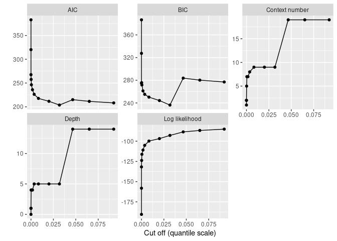
The plot shows that simpler models are too simple as the BIC increases when pruning becomes strong enough. The best model remains rather complex (as expected based on the periodicity of the Solar cycle):
best_sun_model <- as_vlmc(sun_model_tune)
draw(best_sun_model)
#> * (0.5052, 0.4948)
#> +-- high (0.8207, 0.1793)
#> |   +-- high (0.7899, 0.2101)
#> |   |   +-- high (0.7447, 0.2553)
#> |   |   |   +-- high (0.6571, 0.3429)
#> |   |   |   |   '-- low (0.9167, 0.08333)
#> |   |   |   '-- low (1, 0)
#> |   |   '-- low (0.96, 0.04)
#> |   '-- low (0.9615, 0.03846)
#> '-- low (0.1888, 0.8112)
#>     +-- high (0, 1)
#>     '-- low (0.2328, 0.7672)
#>         +-- high (0, 1)
#>         '-- low (0.3034, 0.6966)
#> '-- high (0.07692, 0.9231)To illustrate the use of covariates, we use the power consumption
data set included in the package (see vignette("covlmc")
for details). We consider a week of electricity usage as follows:
pc_week_5 <- powerconsumption[powerconsumption$week == 5, ]
elec <- pc_week_5$active_power
ggplot(pc_week_5, aes(x = date_time, y = active_power)) +
  geom_line() +
  xlab("Date") +
  ylab("Activer power (kW)")
The time series displays some typical patterns of electricity usage:
We build a discrete time series from those (somewhat arbitrary) thresholds:
elec_dts <- cut(elec, breaks = c(0, 0.4, 2, 8), labels = c("low", "typical", "high"))The best VLMC model is quite simple. It is almost a standard order one Markov chain, up to the order 2 context used when the active power is typical.
elec_vlmc_tune <- tune_vlmc(elec_dts)
best_elec_vlmc <- as_vlmc(elec_vlmc_tune)
draw(best_elec_vlmc)
#> * (0.1667, 0.5496, 0.2837)
#> +-- low (0.7665, 0.2335, 0)
#> '-- typical (0.0704, 0.8466, 0.08303)
#> |   '-- low (0.3846, 0.5385, 0.07692)
#> '-- high (0.003497, 0.1573, 0.8392)
As pointed about above, low active power tend to correspond to night phase. We can include this information by introducing a day covariate as follows:
elec_cov <- data.frame(day = (pc_week_5$hour >= 7 & pc_week_5$hour <= 17))A COVLMC is estimated using the covlmc function:
elec_covlmc <- covlmc(elec_dts, elec_cov, min_size = 2, alpha = 0.5)
draw(elec_covlmc, time_sep = " | ", model = "full", p_value = FALSE)
#> *
#> +-- low ([ (I)    | day_1TRUE
#> |          -1.558 | 1.006     ])
#> '-- typical
#> |   +-- low ([ (I)    | day_1TRUE | day_2TRUE
#> |   |          0.3567 | -27.81    | 27.81
#> |   |          -1.253 | -14.39    | 13.69     ])
#> |   '-- typical ([ (I)    | day_1TRUE
#> |   |              2.666  | 0.566
#> |   |              0.2683 | 0.2426    ])
#> |   '-- high ([ (I)    | day_1TRUE
#> |               2.015  | 16.18
#> |               0.6931 | 16.61     ])
#> '-- high ([ (I)   | day_1TRUE
#>             17.41 | -14.23
#>             19.38 | -14.88    ])
The model appears a bit complex. To get a more adapted model, we use a BIC based model selection as follows:
elec_covlmc_tune <- tune_covlmc(elec_dts, elec_cov)
print(autoplot(elec_covlmc_tune))
best_elec_covlmc <- as_covlmc(elec_covlmc_tune)
draw(best_elec_covlmc, model = "full", time_sep = " | ", p_value = FALSE)
#> *
#> +-- low ([ (I)    | day_1TRUE
#> |          -1.558 | 1.006     ])
#> '-- typical
#> |   +-- low ([ (I)
#> |   |          0.3365
#> |   |          -1.609 ])
#> |   '-- typical ([ (I)
#> |   |              2.937
#> |   |              0.3747 ])
#> |   '-- high ([ (I)
#> |               2.773
#> |               1.705 ])
#> '-- high ([ (I)
#>             3.807
#>             5.481 ])
As in the VLMC case, the optimal model remains rather simple:
VLMC models can also be used to sample new time series as in the VMLC
bootstrap proposed by Bühlmann and Wyner. For instance, we can estimate
the longest time period spent in the high active power regime.
In this “predictive” setting, the AIC
may be more adapted to select the best model. Notice that some
quantities can be computed directly from the model in the VLMC case,
using classical results on Markov Chains. See
vignette("sampling") for details on sampling.
We first select two models based on the AIC.
best_elec_vlmc_aic <- as_vlmc(tune_vlmc(elec_dts, criterion = "AIC"))
best_elec_covlmc_aic <- as_covlmc(tune_covlmc(elec_dts, elec_cov, criterion = "AIC"))
The we sample 100 new time series for each model, using the
simulate() function as follows:
set.seed(0)
vlmc_simul <- vector(mode = "list", 100)
for (k in seq_along(vlmc_simul)) {
  vlmc_simul[[k]] <- simulate(best_elec_vlmc_aic, nsim = length(elec_dts), init = elec_dts[1:2])
}set.seed(0)
covlmc_simul <- vector(mode = "list", 100)
for (k in seq_along(covlmc_simul)) {
covlmc_simul[[k]] <- simulate(best_elec_covlmc_aic, nsim = length(elec_dts), covariate = elec_cov, init = elec_dts[1:2])
}Then statistics can be computed on those time series. For instance, we look for the longest time period spent in the high active power regime.
longuest_high <- function(x) {
  high_length <- rle(x == "high")
  10 * max(high_length$lengths[high_length$values])
}
lh_vlmc <- sapply(vlmc_simul, longuest_high)
lh_covlmc <- sapply(covlmc_simul, longuest_high)
The average longest time spent in high consecutively is
The following figure shows the distributions of the times obtained by both models as well as the observed value. The VLMC model with covariate is able to generate longer sequences in the high active power state than the bare VLMC model as the consequence of the sensitivity to the day/night schedule.
lh <- data.frame(
  time = c(lh_vlmc, lh_covlmc),
  model = c(rep("VLMC", length(lh_vlmc)), rep("COVLMC", length(lh_covlmc)))
)
ggplot(lh, aes(x = time, color = model)) +
  geom_density() +
  geom_rug(alpha = 0.5) +
  geom_vline(xintercept = longuest_high(elec_dts), color = 3)
The VLMC with covariate can be used to investigate the effects of changes in those covariates. For instance, if the day time is longer, we expect high power usage to be less frequent. For instance, we simulate one week with a day time from 6:00 to 20:00 as follows.
elec_cov_long_days <- data.frame(day = (pc_week_5$hour >= 6 & pc_week_5$hour <= 20))
set.seed(0)
covlmc_simul_ld <- vector(mode = "list", 100)
for (k in seq_along(covlmc_simul_ld)) {
  covlmc_simul_ld[[k]] <- simulate(best_elec_covlmc_aic, nsim = length(elec_dts), covariate = elec_cov_long_days, init = elec_dts[1:2])
}
As expected the distribution of the longest time spend consecutively in high power usage is shifted to lower values when the day length is increased.
lh_covlmc_ld <- sapply(covlmc_simul_ld, longuest_high)
day_time_effect <- data.frame(
  time = c(lh_covlmc, lh_covlmc_ld),
  `day length` = c(rep("Short days", length(lh_covlmc)), rep("Long days", length(lh_covlmc_ld))),
  check.names = FALSE
)
ggplot(day_time_effect, aes(x = time, color = `day length`)) +
  geom_density() +
  geom_rug(alpha = 0.5)