A Bias Bound Approach to Non-parametric Inference
This is an affiliated package for Susanne M Schennach, A Bias Bound Approach to Non-parametric Inference, The Review of Economic Studies, Volume 87, Issue 5, October 2020, Pages 2439–2472, https://doi.org/10.1093/restud/rdz065
version 0.1.0
Example: See the help documentation of a function
?biasBound_density# Generate sample dataset
X = gen_sample_data(size = 1000, dgp = "2_fold_uniform", seed = 123456)
Y = -X^2 + 3*X + rnorm(1000)*XFor Stata/SAS/SPSS format dataset, one can use the haven package to load the dataset.
# Example for loading the Stata file
library(haven)
sample_data <- read_dta(file.path(EXT_DATA_PATH, "sample_data.dta"))
sample_data
# A tibble: 1,000 × 2
#        X     Y
#    <dbl> <dbl>
#  1 1.09  2.83
#  2 1.63  2.01
#  3 1.23  3.35
#  4 1.07  1.95
#  5 0.844 1.39
#  6 0.879 1.95
#  7 1.49  1.62
#  8 0.699 2.04
#  9 1.38  0.528
# 10 0.866 2.83
# ℹ 990 more rows
# ℹ Use `print(n = ...)` to see more rowsbiasBound_density() functionIf x is specified it will return the point estimation
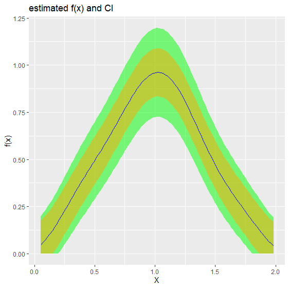
biasBound_density(X = X, x = 1, h = 0.09, alpha = 0.05, if_plot_ft = TRUE, kernel.fun = "Schennach2004")
# $est_Ar
# est_A est_r
# 4.297778 1.998942
#
# $b1x
# [1] 0.1270842
#
# $ft_plot
#
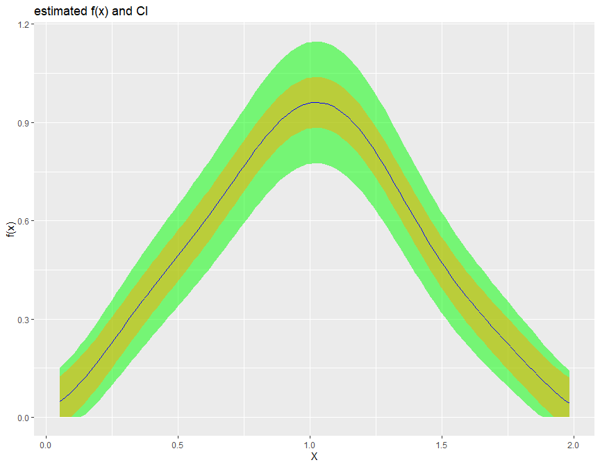
# $f1x
# [1] 0.9598753
#
# $CI
# lb ub
# 0.7245948 1.1951559 If not, it returns the estimation over the whole range of X
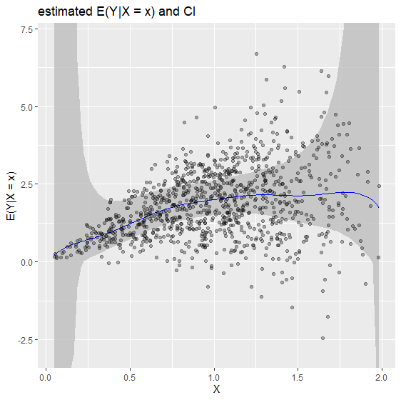
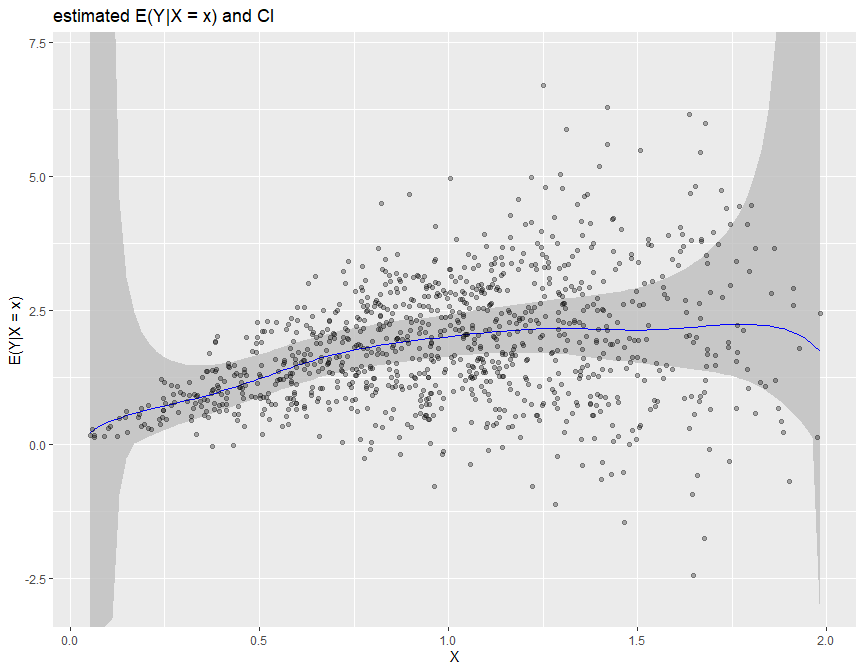
biasBound_condExpectation() functionIf x is specified, it returns the point estimation of \(E(Y|X = x)\)
biasBound_condExpectation(Y = Y, X = X, x = 1, h = 0.09, alpha = 0.05, kernel.fun = "Schennach2004")

# $conditional_mean_yx
# [1] 2.001679
#
# $CI
# lb       ub
# 1.501453 2.609014
If not, it returns the estimation over the whole range of X
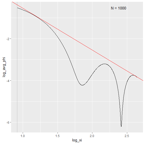
The Fourier Transform frequency \(\xi\) plays an important role in our bias bound approach. Specifically, it determines the range in which a nonparametric estimation the key parameters total variation \(A\) and order of differentiability \(r\) of the unknown distribution function. By default, it is determined by the Theorem 2 in Schennach (2020).
Here is an example how we can customize the range of \(\xi\) when performing the density and conditional expectation estimation.
# Example 1: Specifying x for point estimation with manually selected xi range from 1 to 12
biasBound_density(X = sample_data$X, x = 1, h = 0.09, xi_lb = 1, xi_ub = 12)
# $est_Ar
# est_A est_r
# 5.569499 2.229150
#
# $b1x
# [1] 0.07771575
#
# $ft_plot
# Example 2: Density estimation with manually selected xi range from 1 to 12 xi_lb and xi_ub
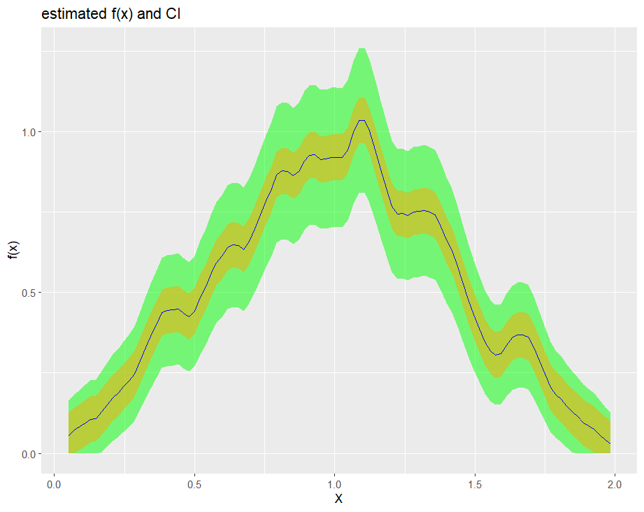
biasBound_density(X = sample_data$X, h = 0.09, xi_lb = 1, xi_ub = 12, if_plot_ft = FALSE)
# Example 3: conditional expectation of Y on X with manually selected range of xi
biasBound_condExpectation(Y = sample_data$Y, X = sample_data$X, h = 0.09, xi_lb = 1, xi_ub = 12)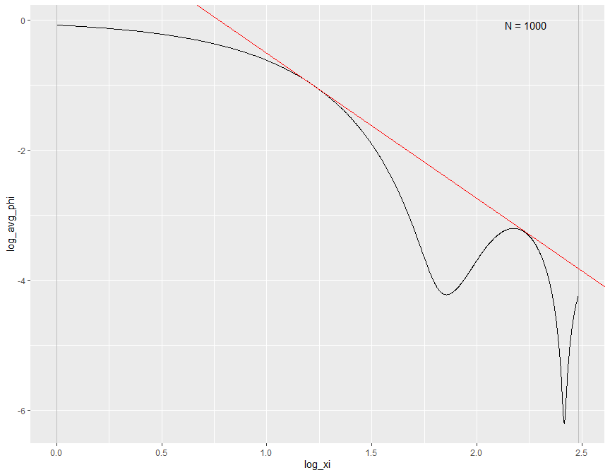
We provide several options for kernel function, such as sinc, normal and epanechnikov kernel.