The goal of shortIRT is to simple tool for the development of static short test forms (STFs) in an Item Response Theory (IRT) based framework. Specifically, two main procedures are considered:
The typical IRT-based procedure for the development of STFs (here denoted as benchmark procedure, BP), according to which the most informative items are selected without considering any specific level of the latent trait
The IRT procedure based on the definition of levels of interest of the latent trait (i.e., \(\theta\) targets, here denoted as \(\theta\)-target procedure). The selected items are those most informative in respect to the \(\theta\) targets. This procedure can be further categorized according to the methodology used for the definition of the \(\theta\) targets:
You can install the development version of shortIRT from GitHub with:
In the example, a 5-item STF is developed from a full-length test of 20 items.
First, generate the responses of 1,000 respondents to the 20 items of the full-length test:
 # Simulate person and item parameters
 true_theta <- rnorm(1000)
 b <- runif(30, -3, 3)
 a <- runif(30, 0.6, 2)
 parameters <- data.frame(b, a)
 # simulate data
 data <- sirt::sim.raschtype(true_theta, b = b, fixed.a = a)
Then, use the EIP for the development of the 5-item STF, including also the matrix of the item parameters and the true \(\theta\) of the subjects (these arguments are not mandatory).
stf_eip <- eip(data, item_par = parameters, starting_theta = true_theta, num_item = 5)
# Show the items included in the STF, the theta targets, and the IIFs of
# the optimal item for each theta target
stf_eip$item_stf
#>     item theta_target item_info stf_length
#> 2    I02      -2.1550 0.6658502      STF-5
#> 52   I22      -1.0295 0.7540494      STF-5
#> 74   I14       0.0915 0.8915867      STF-5
#> 95   I05       1.2110 0.8691818      STF-5
#> 144  I24       2.3350 0.4488457      STF-5
Plot the test information function of both the full-length test and the STF:
plot_tif(stf_eip, tif = "both")  + theme_light() +
  ylab("Information") + xlab(expression(theta)) +
  theme(axis.title = element_text(size = 26),
        strip.text.x = element_text(size = 28))
Now, the bias between the true \(\theta\) and the estimated \(\theta\) (\(\hat{\theta}\)) can be computed as well with the diff_theta() function, which returns both the difference and the absolute difference between \(\theta\)s:
bias_eip <- diff_theta(stf_eip, true_theta = true_theta)
head(bias_eip)
#>   true_theta     stf_theta difference abs_difference
#> 1 -1.2522175 -3.822527e-79 -1.2522175      1.2522175
#> 2  0.6921845  2.936331e-79  0.6921845      0.6921845
#> 3  1.6889284  1.397124e-78  1.6889284      1.6889284
#> 4 -1.6417720 -3.822527e-79 -1.6417720      1.6417720
#> 5  0.6852846  2.952000e-79  0.6852846      0.6852846
#> 6 -1.9871210 -1.462003e-78 -1.9871210      1.9871210
Finally, bias can also be plotted with the function plot_difference() as a function of different levels of \(\theta\). Default is to plot the difference as a function of 4 levels of \(\theta\):
plot_difference(bias_eip) + theme_light() +
  ylab("Difference") + xlab(expression(theta)) +
  theme(axis.title = element_text(size = 26),
        strip.text.x = element_text(size = 28),
         axis.text = element_text(size = 18, angle = 45, hjust=1))
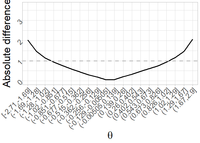
But this can be changed by changing the default of the arguments type and levels to plot, for instance, the absolute difference for 20 levels of the latent trait:
plot_difference(bias_eip, type = "absolute_diff", levels = 20) + theme_light()  + xlab(expression(theta)) +
  theme(axis.title = element_text(size = 26),
        strip.text.x = element_text(size = 28),
        axis.text = element_text(size = 18, angle = 45, hjust=1))