stcpR6: Sequential Test and Change-Point detection algorithms based on E-values / E-detectors

stcpR6 is an R package built to run nonparametric sequential tests and online change point detection algorithms in SRR 21’ and SRR 23’. This package supports APIs of nonparametric sequential test and online change-point detection for streams of univariate sub-Gaussian, binary, and bounded random variables.

Disclaimer: This R package is a personal project and is not affiliated with my company. It is provided “as is” without warranty of any kind, express or implied. The author does not assume any liability for any errors or omissions in this package.

Installation

You can install the development version of stcpR6 from GitHub with:

# install.packages("devtools")
devtools::install_github("shinjaehyeok/stcpR6")

Example

Setup: tracking prediction accuracy.

• Under pre-change, \(Y_t = t + ϵ_t\) for \(t = 1, 2, \dots, \nu\).
• Under post-change, \(Y_t = t + 0.01 * (t-\nu)^2 + ϵ_t\) for \(t = \nu +1, \nu+2, \dots\).
• Prediction: Simple linear regression based on \((t, Y_t)\) history.

Build E-detector on residuals.

We will use E-detector for bounded random variables with the following setup

• Pre-change: Expected residual is equal to zero given sample history.
• Post-change : Expected residual is not equal to zero given sample history.
• Minimum practically interesting gap between pre- and post-means : \(\Delta = 1\).
• Average run length (ARL) level : ARL \(\geq 1000\). i.e., False alert once in 1000 times.
• Cap residuals into \([-20, 20]\).

kCap <- 20 
kARL <- 1000

normalize_obs <- function(y) {
  obs <- (y + kCap) / (2 * kCap)
  obs[obs > 1] <- 1
  obs[obs < 0] <- 0
  return(obs)
}

e_detector <- stcpR6::Stcp$new(
    method = "SR",
    family = "Bounded",
    alternative = "two.sided",
    threshold = log(kARL),
    m_pre = normalize_obs(0),
    delta_lower = 1 / kCap / 2
  )

Case 1. No change happened (Normal condition)

# Set random seed for reproducibility
set.seed(100)
# No change
sig <- 10
v <- 200

y_history <- seq(1,v) + rnorm(v, 0, sig)

# Simple regression predictor
predict_y <- function(i) {
  if (i <= 2) return (0)
  j <- i-1
  coeff <- lm.fit(x = cbind(rep(1, j),1:j), y = y_history[1:j])$coefficients
  return(coeff[1] + coeff[2] * i)
}

y_hat <- sapply(seq_along(y_history), predict_y)

plot(seq_along(y_history), y_history, type = "l", 
xlab = "t", ylab = "Y_t", main = "Sample history (Black) and Prediction (Red)")
lines(seq_along(y_hat), y_hat, col = 2)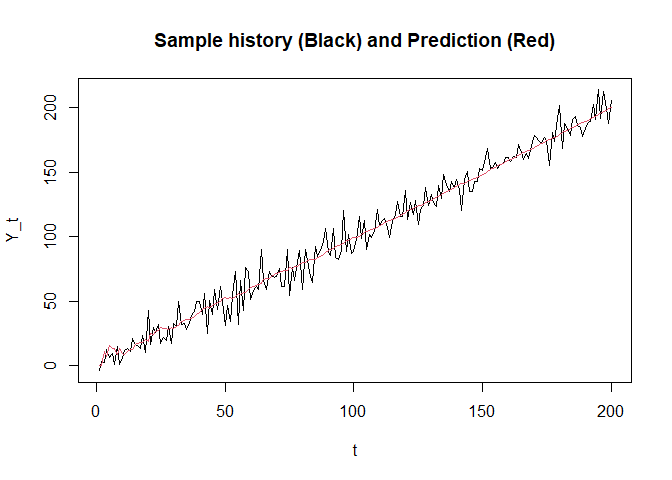

plot(seq_along(y_history), y_history-y_hat, type = "l", 
xlab = "t", ylab = "Residual", main = "Prediction error")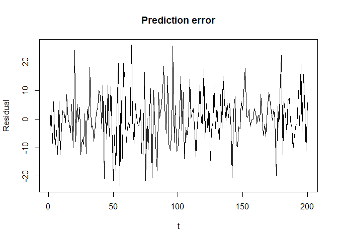

Apply E-detector on normalized residuals

res <- normalize_obs(as.numeric(y_history-y_hat))
# In real applications, 
# we should use e_detector$updateLogValues(res_i) to update e-deetector
# for each newly observed residual res_i.
# In this example, however, we use a vectorized update for simplicity.

# Initialize the model.
e_detector$reset()
# Compute the log values of e-detectors. 
log_values <- e_detector$updateAndReturnHistories(res) 

# Print a summary of updates
print(e_detector)
#> stcp Model:
#> - Method:  SR 
#> - Family:  Bounded 
#> - Alternative:  two.sided 
#> - Alpha:  0.001 
#> - m_pre:  0.5 
#> - Num. of mixing components:  338 
#> - Obs. have been passed:  200 
#> - Current log value:  4.673126 
#> - Is stopped before:  FALSE 
#> - Stopped time:  0

# Plot the log values and stopping threshold
plot(seq_along(log_values), log_values, type = "l",
xlab = "t", ylab = "log value", ylim = c(0, 3 * e_detector$getThreshold()))
abline(h = e_detector$getThreshold(), col = 2)

Note that the log values of e-detector have remained below the threshold. E-detector didn’t trigger any alert.

Case 2. Change happened at t = 100

# Set random seed for reproducibility
set.seed(100)
# Change point: 100
v <- 100

# Pre-change history
y_pre <- seq(1,v) + rnorm(v, 0, sig)

# Post-change history
y_post <- seq(v+1, 2*v) + 0.01 * seq(1,v)^2 + rnorm(v, 0, sig)
y_history <- c(y_pre, y_post)

# Sample history
y_history <- c(y_pre, y_post)

y_hat <- sapply(seq_along(y_history), predict_y)

plot(seq_along(y_history), y_history, type = "l", 
xlab = "t", ylab = "Y_t", main = "Sample history (Black) and Prediction (Red)")
lines(seq_along(y_hat), y_hat, col = 2)
abline(v = v, lty = 2)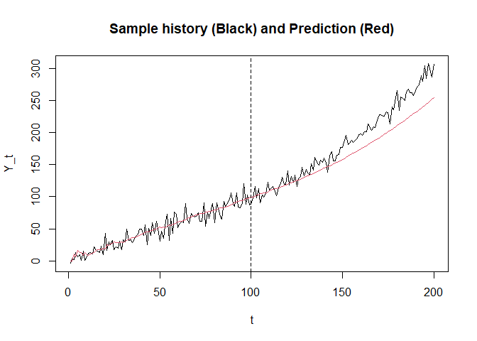

plot(seq_along(y_history), y_history-y_hat, type = "l", 
xlab = "t", ylab = "Residual", main = "Prediction error")
abline(v = v, lty = 2)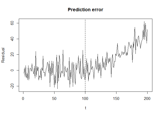

Apply E-detector on normalized residuals

res <- normalize_obs(as.numeric(y_history-y_hat))
# In real applications, 
# we should use e_detector$updateLogValues(res_i) to update e-deetector
# for each newly observed residual res_i.
# In this example, however, we use a vectorized update for simplicity.

# Initialize the model.
e_detector$reset()
# Compute the log values of e-detectors. 
log_values <- e_detector$updateAndReturnHistories(res) 

# Print a summary of updates
print(e_detector)
#> stcp Model:
#> - Method:  SR 
#> - Family:  Bounded 
#> - Alternative:  two.sided 
#> - Alpha:  0.001 
#> - m_pre:  0.5 
#> - Num. of mixing components:  338 
#> - Obs. have been passed:  200 
#> - Current log value:  44.92438 
#> - Is stopped before:  TRUE 
#> - Stopped time:  138

# Plot the log values and stopping threshold
plot(seq_along(log_values), log_values, type = "l",
xlab = "t", ylab = "log value", ylim = c(0, 3 * e_detector$getThreshold()))
abline(h = e_detector$getThreshold() , col = 2)
abline(v = v, lty = 2)
abline(v = e_detector$getStoppedTime(), col = 2, lty = 2)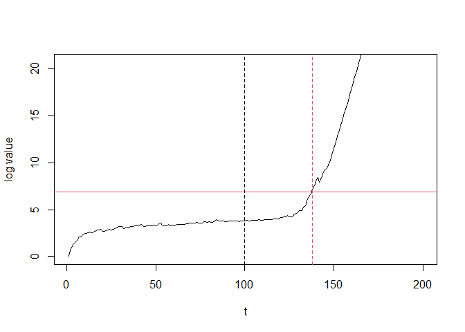

In this case, the log values have crossed the threshold at time 138 and triggered alert. Detection delay was 138 - 100 = 38.

Note that triggering alert at time 138 would be non-trivial if we only check the residual trend as below.

plot(seq_along(y_history), y_history-y_hat, type = "l", 
xlab = "t", ylab = "Residual", main = "Prediction error")
abline(v = v, lty = 2)
abline(v = e_detector$getStoppedTime(), col = 2, lty = 2)