stoppingrule is an R package that provides functionality for constructing, describing, and evaluating stopping rules. Clinical trials often include these rules in order to ensure the safety of study treatments and feasibility of the study.
The current version of stoppingrule is available in this repository. If you have the R package “devtools” installed, stoppingrule can be installed directly from GitHub with:
Suppose a clinical trial of 30 patients is being developed. Study investigators wish to monitor the occurrence of a specific toxicity type, which occurs in 20% of patients in the target population based on historical data. We want to create a stopping rule to test whether the rate of a given toxicity exceeds 20% using a type I error rate of 10%. Moreover, we wish to check the stopping rule continuously, after each patient completes follow-up for the toxicity endpoint.
The function calc.rule.bin creates a ‘rule.bin’ object which contains a matrix with the numbers of evaluable patients and their corresponding stopping boundary values as well as the rule’s design parameters:
require(stoppingrule)
#> Loading required package: stoppingrule
bb_rule = calc.rule.bin(ns=1:30,p0=0.20,alpha=0.10,type="BB",param=c(0.6,2.4))
print(bb_rule)
#> $Rule
#>       N evaluable Reject bdry
#>  [1,]           1           2
#>  [2,]           2           3
#>  [3,]           3           3
#>  [4,]           4           3
#>  [5,]           5           4
#>  [6,]           6           4
#>  [7,]           7           5
#>  [8,]           8           5
#>  [9,]           9           5
#> [10,]          10           5
#> [11,]          11           6
#> [12,]          12           6
#> [13,]          13           6
#> [14,]          14           7
#> [15,]          15           7
#> [16,]          16           7
#> [17,]          17           7
#> [18,]          18           8
#> [19,]          19           8
#> [20,]          20           8
#> [21,]          21           9
#> [22,]          22           9
#> [23,]          23           9
#> [24,]          24           9
#> [25,]          25          10
#> [26,]          26          10
#> [27,]          27          10
#> [28,]          28          10
#> [29,]          29          11
#> [30,]          30          11
#>
#> $ns
#>  [1]  1  2  3  4  5  6  7  8  9 10 11 12 13 14 15 16 17 18 19 20 21 22 23 24 25
#> [26] 26 27 28 29 30
#>
#> $p0
#> [1] 0.2
#>
#> $type
#> [1] "BB"
#>
#> $alpha
#> [1] 0.1
#>
#> $param
#> [1] 0.6 2.4
#>
#> $cval
#> [1] 0.9630823
#>
#> attr(,"class")
#> [1] "rule.bin"
The function call uses the Bayesian beta-binomial model approach proposed by Geller et al. 2003 to construct the stopping boundaries and displays the boundaries for the first few patients. A weakly informative Beta(0.6,2.4) is specified for the toxicity probability. The `bb_rule$Rule’ element of the output displays the number evaluable and stopping criteria for all analyses; other elements contain the design parameters and boundary parameter for the stopping rule. For this rule, rejection is impossible with 1 or 2 evaluable patients because the corresponding boundary values exceeds these numbers.
The function table.rule.bin can produce a succinct summary of the stopping rule for the entire cohort from the rule calculated above:
table.rule.bin(bb_rule)
#> N evaluable Reject If N >=
#> [1,] "3 - 4" "3"
#> [2,] "5 - 6" "4"
#> [3,] "7 - 10" "5"
#> [4,] "11 - 13" "6"
#> [5,] "14 - 17" "7"
#> [6,] "18 - 20" "8"
#> [7,] "21 - 24" "9"
#> [8,] "25 - 28" "10"
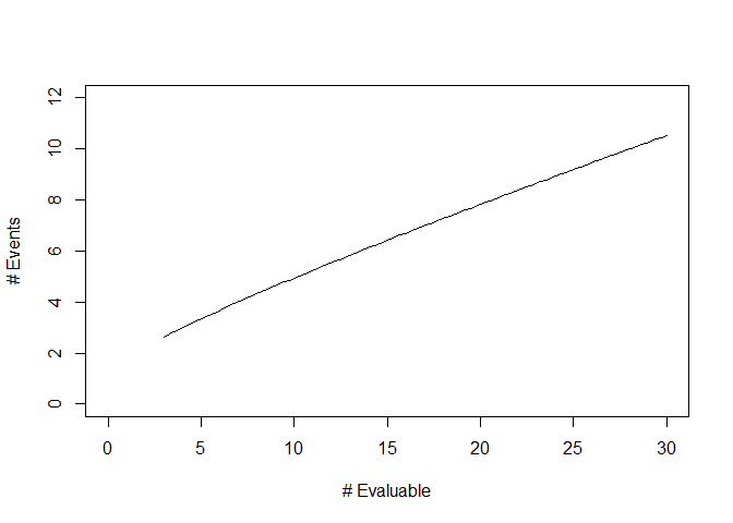
#> [9,] "29 - 30" "11"We can also obtain a graphical summary of the stopping rule using the plot function:
Lastly, the OC.rule.bin function can assess the operating characteristics of this stopping rule. The rejection probability and expected numbers of events at the time of stopping are computed at true toxicity rates of p = 20%, 25%, 30%, 35%, and 40% as follows: