Surveyexplorer

Visualize and tabulate single-choice, multiple-choice, matrix-style questions from survey data. Includes ability to group cross-tabulations, frequency distributions, and plots by categorical variables and to integrate survey weights. Ideal for quickly uncovering descriptive patterns in survey data.

Installation

# install.packages("devtools"), if not already downloaded
devtools::install_github("liamhaller/surveyexplorer")

Examples

library(surveyexplorer)

The data used in the following examples is from the berlinbears dataset, a fictional survey of bears in Berlin, that is included in the surveyexplorer package.

Single-choice questions

#Basic table
single_table(berlinbears, 
             question = income)

Use group_by = to partition the question into several groups

single_table(berlinbears,
             question = income,
             group_by = gender)

Ignore unwanted subgroups with subgroups_to_exclude

single_table(berlinbears,
             question = income, 
             group_by = gender, 
             subgroups_to_exclude = NA) 

Remove NAs from the question variable with na.rm

single_table(berlinbears,
             question = income, 
             group_by = gender, 
             subgroups_to_exclude = NA,
             na.rm = TRUE)

Finally, you can specify survey weights using the weight option

single_table(berlinbears,
             question = income, 
             group_by = gender, 
             subgroups_to_exclude = NA,
             na.rm = TRUE,
             weights = weights)

The same syntax can be applied to the single_freq function to plot frequencies of the question optionally partitioned by subgroups.

single_freq(berlinbears,
             question = income, 
             group_by = gender, 
             subgroups_to_exclude = NA,
             na.rm = TRUE,
             weights = weights)

Multiple-choice questions

The options and syntax for multiple-choice tables multi_table and graphs multi_graphs are the same. The only difference is the question input also accommodates tidyselect syntax to select several columns for each answer option. For example, the question “will_eat” has five answer options each prefixed by “will_eat”

berlinbears |> 
  dplyr::select(starts_with('will_eat')) |> 
  head()
#>   will_eat.SQ001 will_eat.SQ002 will_eat.SQ003 will_eat.SQ004 will_eat.SQ005
#> 1              0              1              0              1              1
#> 2              0              1              1              1              1
#> 3              1              1              0              1              1
#> 4              0              0              0              1              0
#> 5              0              0              0              1              1
#> 6              0              0              0              1              0

The same syntax can be used to select the question for the multiple choice tables and graphs

multi_table(berlinbears, 
            question = dplyr::starts_with('will_eat'), 
            group_by = genus, 
            subgroups_to_exclude = NA,
            na.rm = TRUE)

For graphing, the multi_freq function creates an UpSet plot to visualize the frequencies of the intersecting sets for each answer combination and also includes the ability to specify weights.

multi_freq(berlinbears, 
            question = dplyr::starts_with('will_eat'), 
            na.rm = TRUE,
            weights = weights)
#> Estimes are only preciese to one significant digit, weights may have been rounded

The graphs can also be grouped

multi_freq(berlinbears, 
            question = dplyr::starts_with('will_eat'), 
            group_by = genus,
            subgroups_to_exclude = NA,
            na.rm = FALSE,
            weights = weights)
#> Estimes are only preciese to one significant digit, weights may have been rounded

Matrix Questions

matrix_table has the same syntax as above and works with array or categorical questions

matrix_table(berlinbears, 
             dplyr::starts_with('p_'),
             group_by = is_parent)
matrix_table(berlinbears, 
             dplyr::starts_with('c_'),
             group_by = is_parent)

matrix_freq visualizes the frequencies of responses

matrix_freq(berlinbears, 
             dplyr::starts_with('p_'))

matrix_freq(berlinbears, 
             dplyr::starts_with('c_'),
             group_by = is_parent)

For array/matrix style questions that are numeric matrix_mean plots the mean values and confidence intervals

matrix_mean(berlinbears, 
             question = dplyr::starts_with('p_'),
             na.rm = TRUE)

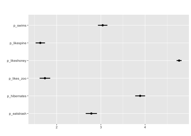
#Can also apply grouping
matrix_mean(berlinbears, 
            question = dplyr::starts_with('p_'),
            na.rm = TRUE,
            group_by = species, 
            subgroups_to_exclude = NA)

#with survey weights
matrix_mean(berlinbears, 
            question = dplyr::starts_with('p_'),
            na.rm = TRUE,
            group_by = species, 
            subgroups_to_exclude = NA, 
            weights = weights)

Finally, for Likert questions (scales of 3,5,7,9…) matrix_likert provides a custom plot

matrix_likert(berlinbears, 
              question = dplyr::starts_with('p_'))

#you can specify custom labels with the `label` argument
matrix_likert(berlinbears,
              question = dplyr::starts_with('p_'),
              labels = c('Strongly disagree', 'Disagree','Neutral','Agree','Strongly agree'))

#and pass colors using the colors option 
matrix_likert(berlinbears, 
              question = dplyr::starts_with('p_'),
              labels = c('Strongly disagree', 'Disagree','Neutral','Agree','Strongly agree'),
              colors = c("#E1AA28", "#1E5F46", "#7E8F75", "#EFCD83", "#E17832"))

#can also apply weights 
matrix_likert(berlinbears, 
              question = dplyr::starts_with('p_'),
              labels = c('Strongly disagree', 'Disagree','Neutral','Agree','Strongly agree'), 
              colors = c("#E1AA28", "#1E5F46", "#7E8F75", "#EFCD83", "#E17832"),
              weights = weights) 

Overview

Functions

• Single-choice
  • single_table
  • single_freq
• Multiple-choice
  • multi_table
  • multi_freq
• Matrix
  • matrix_table
  • matrix_freq
  • matrix_mean
  • matrix_likert

*_table functions return a gt table of the cross tabulations and frequencies for each question while *_freq returns the same data but as a plot.

For matrix-style questions with numerical input, matrix_mean plots the mean value value and ± two standard deviations. matrix_likert visualizes questions that accept Likert responses (strongly agree-strongly disagree) or questions with 3,5,7,9… categories.

Syntax

Each function contains the following options

• dataset —The input dataframe (or tibble) of survey questions
• question — The column(s) that contain the response options for a question, can be selected by using tidyselect semantics or providing a vector of column names or numbers
• group_by — Optional variable to group the analysis. If provided, the frequencies and counts will be calculated within each subgroup
• subgroups_to_exclude — Optional vector specifying subgroups to exclude from the analysis
• weights — Optional variable containing survey weights. If provided, frequencies and counts will be weighted accordingly
• na.rm — Logical indicating whether to remove NA values from question before analysis